In this post we outline our method, \(TRAK\ W_{ith}\ O_{ptimally}\ M_{odified}\ P_{rojections}\), which sets a new SOTA for predicting the downstream effects of dataset changes!
At Womp Labs, we spend all of our time thinking about the way ML models use their training data. When a model fails, it would be great to pinpoint the source of the problem. When you have many data sources, you’d like to know if only one of them was doing the heavy lifting.
Anyone training models knows there is still a fair amount of witchcraft that goes into turning chunks of tokens into sensible, useful things. Some of this is interpretable, like the fact that coding examples help with logic and reasoning problems. Some of it, like the fact that math examples can break safety guardrails, is less so. And it becomes even more complicated when you consider that these heuristics are dependent on the model you’re training and the other data at your disposal. For these reasons, it becomes increasingly important to work on ways to quantify what data points are actually contributing to a training run.
The methods used to solve these problems fall under the umbrella of data attribution. Fundamentally, this is a challenge of tracing model outputs to training data, and then using this understanding to infer how to change data to affect downstream behavior. Some background can be found in this ICML tutorial.
A core goal is to accurately predict the outcome of training on some dataset without having to do so. To quantify how good a method is at this, we can use the following:
\[LDS(\tau,z):=\rho(f(z,\theta^*(D_j)):j\in[m],{g_\tau(z,D_j;D):j\in[m]})\tag{1}\]
where \(D\) is the training set, \(f\) is the output of model \(\theta^*\), trained on \(D_j\subset D\), on an example of interest \(z\), \(m\) is number of evaluation subsets, \(g_\tau\) is the output prediction made by attribution method \(\tau\), and \(\rho\) is the spearman correlation. In simpler terms, we are trying to answer the following question:
\[How\ accurately\ can\ we\ predict\ which\ dataset\ is\ better\ for\ learning\ example\ z?\]
Just over a year ago, a lab at MIT introduced TRAK, a data attribution method orders of magnitudes more efficient than the prior state of the art. Their approach casts the complex problem of attributing influence in neural nets to the well understood setting of linear regression. Leaving the details to their paper, the final form of their method is as follows:
\[\tau_{TRAK}(z,S) := S(\frac{1}{M^2}(\sum_{m=1}^M Q_m)*(\sum_{m=1}^M\phi_m(z)(\Phi_m^T\Phi_m)^{-1}\Phi_m^T),\hat\lambda)\tag{2}\]
where \(z\) is an example of interest, \(M\) is the number of reference models used, \(\phi\) is a random projection of \(\nabla_\theta f(z)\), \(\Phi\) is the stacked matrix of \(\phi(x)\) for all training examples \(x\), \(Q\) is the diagonal matrix of \(1-p_i\) with \(p_i\) being the predicted correct-class probability of \(x_i\) at \(\theta^*\), and \(S\) is a soft threshold function with threshold \(\hat\lambda\).
One of the understood sources of error in the TRAK formulation is the random projection step. However, a theoretical result from Johnson and Lindenstrauss, which shows inner products are preserved with high probability when projecting via a matrix \(P\sim\mathcal{N}(0,1)^{p\times{k}}\), leads to the belief that this error is small. As a result, the improvement from ensembling \(M\) different models is attributed to the need for different training trajectories to sample different possible loss landscapes.
We show that this is not entirely the case. In fact, a large portion of the error comes from imperfections in the projection step.
To reduce this degradation in accuracy, one can increase the projection dimension. But, the TRAK paper shows there is an optimal projection dimension, beyond which performance starts to degrade. While we expect higher-dimensional representations to be less lossy, the issue comes from the inverse Hessian approximation \((\Phi_m^T\Phi_m)^{-1}\). As dimensionality increases, the number of spurious correlations grows. But, a small tweak to the setup fixes this problem.
We modify TRAK by decomposing the projected gradients into blocks. In doing so, we produce what resembles multiple checkpoints from a single backward pass. For example, one checkpoint projected to \(d=4096\) can also be treated as \(4\) different \(d_{batch}=1024\) checkpoints. The result is the following formulation:
\[\tau_{TRAK_{WOMP}}(z,S) := S(\frac{1}{M^2}(\sum_{m=1}^M Q_m)*(\sum_{m=1}^M\sum_{b=1}^B\phi_{m,b}(z)(\Phi_{m,b}^T\Phi_{m,b})^{-1}\Phi_{m,b}^T),\hat\lambda)\tag{3}\]
where \(B\) is the number of blocks we decompose the projection into and \(\phi_{m,b}(z)\) is the \(b^{th}\) block of \(\phi_{m}(z)\).
An alternative way to frame our setup is as a block-wise decomposition of the \(H^{-1}\) approximation. We redefine this term as:
\[\hat{H}_m^{-1} := diag(\Phi_{m,1}^T\Phi_{m,1},\Phi_{m,2}^T\Phi_{m,2},...,\Phi_{m,B}^T\Phi_{m,B})^{-1}\tag{4}\]
Finally, equivalent to \((3)\), we come to the definition:
\[\tau_{TRAK_{WOMP}}(z,S) := S(\frac{1}{M^2}(\sum_{m=1}^M Q_m)*(\sum_{m=1}^M\phi_{m}(z){\hat{H}_m}^{-1}\Phi_{m}^T),\hat\lambda)\tag{5}\]
Our simple change allows us to increase the projection dimension, thereby achieving higher resolution representations, without sacrificing the accuracy of the Hessian approximation. What is nice about this setup is it introduces no additional backward passes per reference model.
This lets us make better predictions without multi-million dollar donations to NVIDIA!
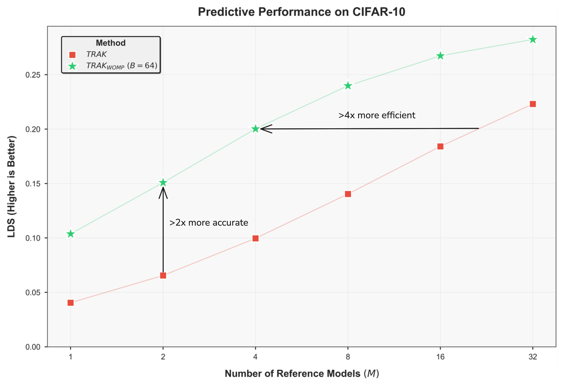
Our goal is to accurately predict the result of training a \(Resnet-9\) on a given subset of \(CIFAR10\) without having to train the model. To make these predictions we train \(M\) models on random \(50\%\) subsets of the dataset. We use checkpoints from these models as reference models to compute attribution scores. We then evaluate the methods with \(LDS\) using \(10,000\) models.
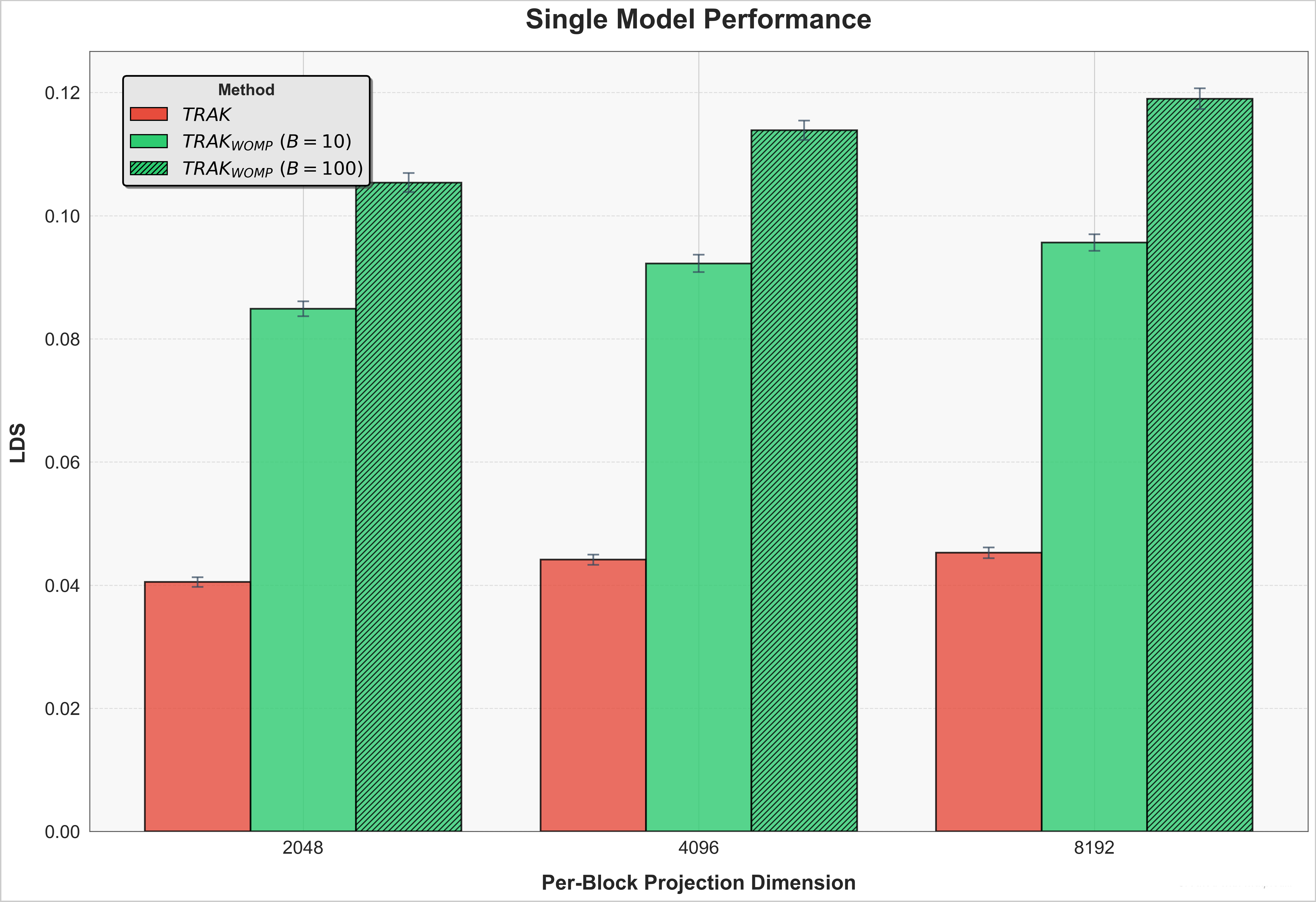
In most settings it is not feasible to retrain multiple models. As a result, the most important measure of effectiveness is the performance when only using \(M=1\) model. We show that \(TRAK_{WOMP}\) drastically outperforms vanilla \(TRAK\).
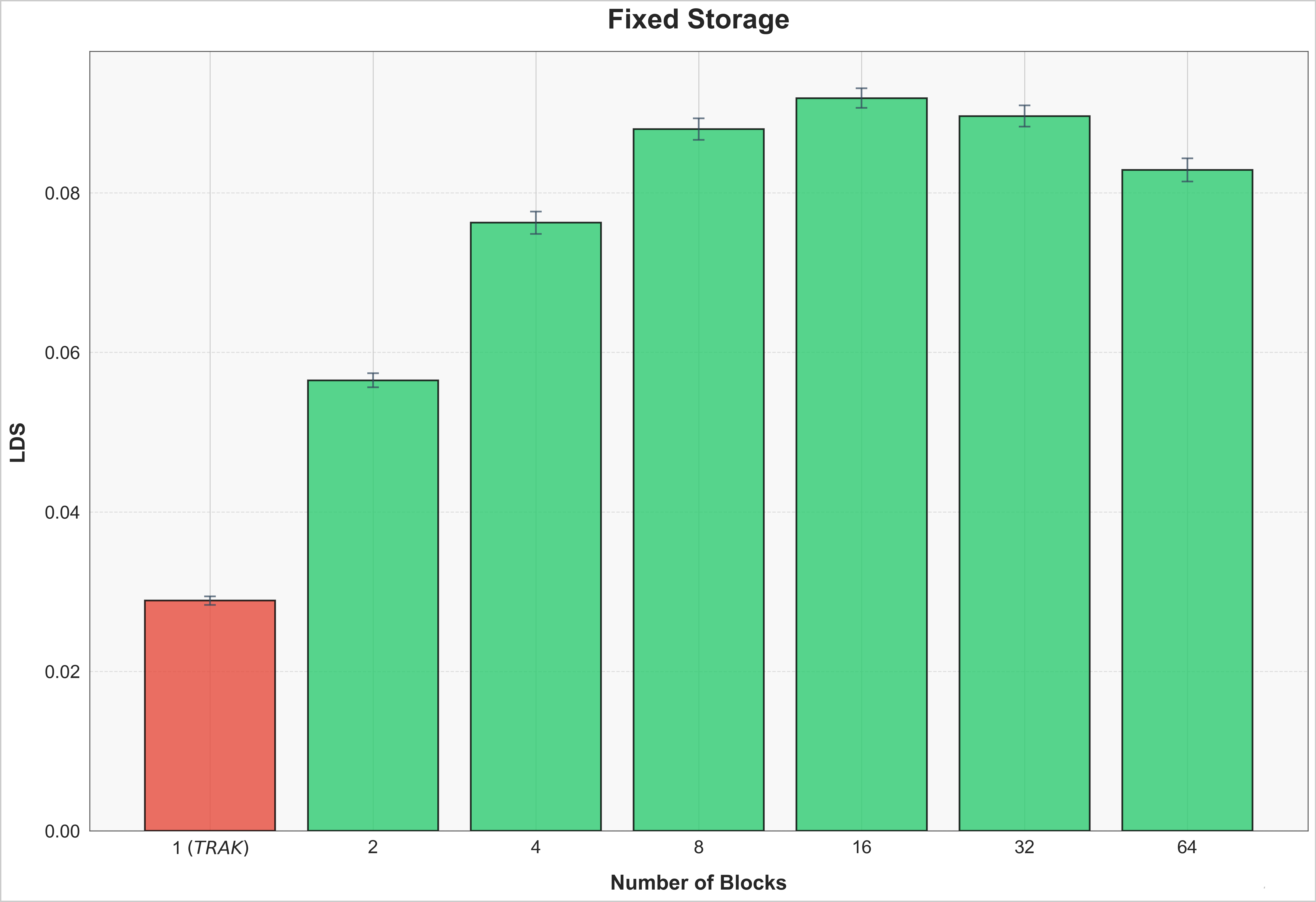
So far, we have shown results when per-block projection dimension was fixed. However, we know this requires \(B\) times more storage. In some cases there can be storage constraints as well. In Figure 3, we fix the total projection dimension, \(d\), and vary \(B\). Our results show that not only is \(TRAK_{WOMP}\) superior on a fixed compute budget, it is better on a fixed storage budget as well.
We know these results are on a small scale model, but we have more to share soon on billion(s) parameter models and internet scale datasets. We believe we can eliminate the hope and guesswork when training large models. If you agree and are interested in collaborating or joining the team, please reach us at contact@womplabs.ai! If you would like to stay up to date on our work, sign up here.
See you next time 🙂
Aug 28, 2024